A unifying view of linear attention

TL;DR

Softmax attention and sub-quadratic models like linear attention belong to the same class of models that make choices across four axes: how to store associative memory (memory architecture), which objective we try to optimize (objective), how to optimize (optimizer), and how to forget (retention). In this setting, we show that softmax attention is a degenerate case where we append everything to memory without any compression, optimization, or forgetting — for which we pay an unbounded KV cache and quadratic attention compute. Sub-quadratic models approximate this perfect recall by having a fixed-size memory and a tiny model that is trained online inside the forward-pass, with specific choices on the memory architecture, objective, optimizer and retention. We derive the finite-state recurrence by replacing the softmax similarity in attention with a finite-dim kernel, which allows us to factor out a fixed-size state matrix. By generalizing this further into $S_t = S_{t-1} A_t + b_t k_t^\top$ we show how specific choices for $A_t$ and $b_t$ influence the four axes and where popular models are placed across them.

1. Setup

Transformers are currently THE default architecture for any foundational model as they can attend to the entire context and thus have perfect recall, and they can be trained very efficiently. But that recall is paid for with an unbounded KV cache (that grows linearly with context) and quadratic compute. Today’s workloads already strain our compute resources and will keep doing that because, as those models get better, we start giving them longer tasks on more context. Tomorrow’s 10–100M context sizes aren’t reachable with this, even with optimizations like Flash Attention, MQA/GQA, or KV compression; they buy us some time but they don’t bend the quadratic curve. So, planning ahead, we should ask: can we get excellent recall from a fixed-size state that is as good (or even better) as softmax attention, but with linear compute? And, will we even need softmax attention in the future?

2. Linear attention

Starting with the familiar equations for softmax attention.

$$\begin{aligned} O &= \mathrm{softmax}(QK^\top \odot M)\,V &&\in \mathbb{R}^{L \times d_v} \\ o_t &= \sum_{j=1}^{t} \frac{\exp(q_t^\top k_j)}{\sum_{l=1}^{t} \exp(q_t^\top k_l)}\, v_j &&\in \mathbb{R}^{d_v} \end{aligned}$$

where $Q$, $K$ and $V$ are the usual query, key and value matrices, with $M$ being the causal mask matrix to ensure tokens cannot attend into the future. Assume that the scaling $1/\sqrt{d}$ is already folded into $q$ for clarity.

Replace $\exp$ with a general function $f$ that measures the similarity between $q$ and $k$:

$$o_t = \sum_{j=1}^{t} \frac{f(q_t, k_j)}{\sum_{l=1}^{t} f(q_t, k_l)}\, v_j \;\in \mathbb{R}^{d_v}.$$

The plain dot product $f(q,k) = q^\top k$ is one widely used choice.

We call $f$ a kernel if there is a $\phi$ such that $f(q, k) = \langle \phi(q), \phi(k) \rangle$. Having a kernel as our similarity function allows us to factor the query-dependent term out of the sum:

$$\begin{aligned} \sum_{j=1}^{t} \big[\phi(q_t)^\top \phi(k_j)\big]\, v_j &= \sum_{j=1}^{t} v_j\, \big[\phi(k_j)^\top \phi(q_t)\big] \\ &= \Big(\sum_{j=1}^{t} v_j\, \phi(k_j)^\top\Big)\, \phi(q_t) \\ &= S_t\, \phi(q_t) \end{aligned}$$

The same factoring applied to the denominator gives

$$o_t = \frac{S_t\, \phi(q_t)}{z_t^\top \phi(q_t)}, \qquad z_t = \sum_{j=1}^{t} \phi(k_j) \;\in \mathbb{R}^{d_\phi}.$$

Modern variants drop the denominator because it can introduce numerical instabilities and we already use normalisation like RMSNorm on the block/layer output anyway; additionally, we get some guarantees later on with gating that bounds $S$. Footnote: (Katharopoulos et al., 2020) Transformers are RNNs: Fast Autoregressive Transformers with Linear Attention Katharopoulos, Vyas, Pappas, Fleuret · ICML 2020 arXiv:2006.16236 keeps $z_t$.

Dropping the denominator and incrementing $t \to t-1$ inside the sum gives the linear-attention recurrence:

$$\boxed{\,S_t = S_{t-1} + v_t\, \phi(k_t)^\top, \qquad o_t = S_t\, \phi(q_t)\,}$$

Each step writes a rank-1 matrix (the outer product of $v_t$ and $\phi(k_t)$) into a fixed-size state $S_t$ of dimension $d_v \times d_\phi$. Total cost per token: $O(d_v d_\phi)$ regardless of sequence length.

Why softmax can’t fit this form. We mentioned that we want a similarity function that is a kernel with $f(q, k) = \langle \phi(q), \phi(k) \rangle$. The good thing is that softmax $f(q,k) = \exp(q^\top k)$ is also a kernel, the only problem is that its feature map $\phi$ is infinite-dimensional, so $S_t$ would be an infinite matrix we cannot materialize. To get a finite-state recurrence we have to pick a kernel with finite-dim $\phi$. (Katharopoulos et al., 2020) Transformers are RNNs: Fast Autoregressive Transformers with Linear Attention Katharopoulos, Vyas, Pappas, Fleuret · ICML 2020 arXiv:2006.16236 chose $\phi(x) = \mathrm{elu}(x) + 1$. That’s the original “linear attention”.

Most follow-up papers skip the feature map and take $\phi(k) = k$ directly, without an explicit softmax-style weighted sum anymore. Generalizing it further, we can write

$$\boxed{\,S_t = S_{t-1}\, A_t + b_t\, k_t^\top\,}$$

where (by convention) $k_t$ stands for whatever key-side vector the model writes — $\phi(W_k x_t)$ for linear attention, or $W_k x_t$ directly. $A_t$ governs what we keep from the previous state and $b_t \in \mathbb{R}^{d_v}$ is the value being written at step $t$. For linear attention it’s $A_t = I$ and $b_t = v_t$.

3. Associative memory

But what is our goal again? With softmax or linear attention we want to retrieve the value $v_i$ for some pair $(k_i,v_i)$ that we have seen already, what we usually refer to as part of our context.

The linear-attention read-out with a query key $k_q$ is:

$$S_t\, k_q \;=\; \sum_{i=1}^{t} v_i\, (k_i^\top k_q)$$

We can split the sum into our signal which we want to retrieve and some cross-talk/noise (here we assume $k_q$ matches some stored key $k_j$ exactly, with $q = j$):

$$S_t\, k_q \;=\; \underbrace{v_q\, \|k_q\|^2}_{\text{signal}} \;+\; \underbrace{\sum_{i \neq q} v_i\, (k_i^\top k_q)}_{\text{cross-talk}}$$

The cross-talk term is what determines whether the recurrence can faithfully store many key–value pairs. If it gets bigger than the signal we won’t be able to retrieve $v_q$.

In practice we want to approximate retrieval, such that similar queries should retrieve similar values:

$$S_t\, k_q \;\approx\; v_q \qquad \text{whenever } k_q \approx k_j \text{ for some stored } j$$

The easy way to achieve this goal is to keep every $(k_i, v_i)$ pair around like softmax does:

$$o_t \;=\; \sum_{i=1}^{t} v_i \cdot \frac{\exp(k_i^\top q_t)}{\sum_{l=1}^{t} \exp(k_l^\top q_t)}$$

As we keep all $t$ past key and value vectors of dimension $d_k$ and $d_v$ respectively, the KV cache size grows linearly with $t$:

$$|\text{KV cache}| \;=\; t \,(d_k + d_v)$$

Linear attention compresses that into a fixed-size $S$, where the compression has a capacity ceiling at $\sim d_k$ stored key-value pairs:

$$\boxed{\;n \,\lesssim\, d_k \quad \text{for reliable recall.}\;}$$

Why linear attention has capacity $\sim d_k$

This shows up cleanly in two limit cases.

Orthogonal-key case (hard cap). If the stored keys are mutually orthogonal — $k_i^\top k_j = 0$ for $i \neq j$ and $\|k_i\| = 1$ — then the cross-talk vanishes and the read-out is exact:

$$k_i^\top k_q = \delta_{iq} \quad\Longrightarrow\quad S_t\, k_q = v_q$$

But $\mathbb{R}^{d_k}$ holds at most $d_k$ mutually orthogonal vectors. So in this regime the recurrence stores at most $d_k$ key-value pairs perfectly. That’s the hard cap.

Random-key case (soft cap, JL concentration). In practice the keys aren’t exactly orthogonal but rather whatever the model produces, and on average behave like random vectors. Take $k_i$ with i.i.d. entries $\mathcal{N}(0, 1/d_k)$. Each pairwise dot product has zero mean and variance $1/d_k$ (follows from Johnson–Lindenstrauss concentration):

$$\mathbb{E}[k_i^\top k_q] = 0, \qquad \operatorname{Var}(k_i^\top k_q) = \frac{1}{d_k}$$

The cross-talk term is a sum of $n-1$ approximately-independent contributions, so its variance adds:

$$\mathbb{E}\|\epsilon\|^2 \;=\; \mathbb{E}\left\| \sum_{i \neq q} v_i\, (k_i^\top k_q) \right\|^2 \;=\; \sum_{i \neq q} \frac{\|v_i\|^2}{d_k} \;=\; \frac{n-1}{d_k}$$

(taking unit-norm values for clarity). The signal-to-noise ratio of the read-out is then

$$\mathrm{SNR} \;=\; \frac{\|v_q\|}{\|\epsilon\|} \;\sim\; \sqrt{\frac{d_k}{n-1}}$$

so $\mathrm{SNR} \sim 1$ exactly when $n \sim d_k$. That’s the regime where retrieval starts breaking down.

The conclusion in both cases: linear attention can store roughly $d_k$ key-value pairs before cross-talk overwhelms the signal.

Putting that together we can look at the compression ratio between softmax attention and linear attention:

$$\frac{|\text{KV cache}|}{|S|} \;=\; \frac{t\,(d_k + d_v)}{d_k\, d_v} \;\approx\; \frac{2t}{d} \quad (\text{with } d_k = d_v = d)$$

The interesting regime is $t \gg d$, when the context is considerably larger than the dimension of our keys/values, and where every sub-quadratic recurrence model is forced to throw information away. The rest of the post is how to do that intelligently by increasing the effective capacity of $S$ and managing what gets forgotten. Different choices of $A_t$ (how the past decays) and $b_t$ (what the new write is) give different architectures.

4. Delta rule

Why we need a smarter write. Recall that linear attention writes

$$S_t = S_{t-1} + v_t\, k_t^\top$$

even when the past state already returns the right value at $k_t$ (i.e. $S_{t-1} k_t = v_t$). Writing the same $(k, v)$ twice doubles the stored value at $k$, amplifying cross-talk for every other key without adding any new information.

So what if we correct rather than just accumulate? The simplest objective for "$Sk \approx v$" would be to just do one step of gradient descent on the L2 loss:

$$L_t(S) = \tfrac{1}{2}\, \|v_t - S k_t\|^2$$

For it we can compute the gradient w.r.t. $S$ in closed-form:

$$\nabla_S L_t \;=\; -(v_t - S k_t)\, k_t^\top \;\in\; \mathbb{R}^{d_v \times d_k}$$

This is just the outer product of the residual $v_t - S k_t$ (how wrong the current read-out at $k_t$ is) and the key $k_t$. Shape-wise it matches $S$, so we can take one gradient step from $S_{t-1}$ with a step size $\beta_t$:

$$S_t \;=\; S_{t-1} + \beta_t\, (v_t - S_{t-1} k_t)\, k_t^\top.$$

Regrouping the $S_{t-1}$ terms gives us the delta rule:

$$\boxed{\,S_t \;=\; S_{t-1}\bigl(I - \beta_t\, k_t k_t^\top\bigr) + \beta_t\, v_t\, k_t^\top\,}$$

So comparing it with our general formula, DeltaNet (Yang et al., 2024) Parallelizing Linear Transformers with the Delta Rule over Sequence Length Yang, Wang, Zhang, Shen, Kim · NeurIPS 2024 arXiv:2406.06484 is the choice $A_t = I - \beta_t k_t k_t^\top$ and $b_t = \beta_t v_t$.

What does $(I - \beta_t k_t k_t^\top)$ actually do? Assuming $\|k_t\| = 1$ (in practice enforced by some normalization on the keys), $k_t k_t^\top$ is the projector onto the line spanned by $k_t$, so $I - \beta_t k_t k_t^\top$ shrinks any component along $k_t$ by a factor of $(1-\beta_t)$ and leaves anything orthogonal to $k_t$ untouched.

To make this concrete, let’s look at the read-out at the just-written key. Writing $v_t^{\text{old}} \equiv S_{t-1} k_t$ for whatever was stored at $k_t$ before the write, we get

$$S_t\, k_t \;=\; (1-\beta_t)\, v_t^{\text{old}} \;+\; \beta_t\, v_t,$$

i.e. a convex blend of the old and new value. With $\beta_t = 1$ the write fully overwrites whatever was there; with $\beta_t = 0$ we ignore the new write. And the read-out at any orthogonal key $k'$ (with $k_t^\top k' = 0$) is just

$$S_t\, k' \;=\; S_{t-1}\, k',$$

completely unchanged. So writing at $k_t$ does not affect the read-out of exactly orthogonal keys.

In practice $\beta_t$ is per-token learnable, something like $\beta_t = \sigma(W_\beta x_t)$. The model can learn to assign small $\beta_t$ to input patterns that tend to be redundant (like filler-words) and large $\beta_t$ to patterns that tend to carry new information (like nouns).

Capacity is unchanged; what’s still missing. We get perfect read-out only when the stored key is exactly orthogonal to $k_t$. The read-out at $k_{\text{old}}$ after the write of a new $k_{\text{new}}$ is

$$S_t\, k_{\text{old}} \;=\; S_{t-1}\, k_{\text{old}} \;-\; \beta_t\,(S_{t-1}\, k_{\text{new}})\cos\theta \;+\; \beta_t\, v_{\text{new}}\, \cos\theta, \qquad \cos\theta \,\equiv\, k_{\text{new}}^\top k_{\text{old}}.$$

When $S$ is crowded — we’ve already stored many key–value pairs — a new key $k_{\text{new}}$ won’t be orthogonal to all of them. For any stored $k_{\text{old}}$ with $\cos\theta$ noticeably non-zero, the equation above says the read-out at $k_{\text{old}}$ gets partially overwritten too: the second term scales down a $\cos\theta$-piece of what was stored along $k_{\text{new}}$, and the third term adds a $\cos\theta$-piece of the new $v_{\text{new}}$. So we end up with the same capacity ceiling as linear attention: DeltaNet still saturates around $n \sim d_k$.

What DeltaNet does fix is the what we write: blind addition becomes an error-correcting write whose size is proportional to how wrong the current read-out at $k_t$ is. Concretely, writing the same $(k, v)$ twice is now a near no-op (the residual is already small on the second write), where linear attention would just double the value at $k$ and amplify the cross-talk.

What it does not fix is the what we forget. The $(I - \beta_t k_t k_t^\top)$ partial-projects only along $k_t$, so anything orthogonal to $k_t$ in $S$ is preserved exactly. A stale write from many steps ago in some direction $k_{\text{old}}$ stays in $S$ at full magnitude forever, unless we happen to write near $k_{\text{old}}$ again. DeltaNet never forgets, so let’s change that with gating.

Figure 1. Updated for DeltaNet:

Model	$A_t$	$b_t$	$\phi$
Softmax	— (no finite $S$)	—	$\exp$ (infinite-dim)
Linear attention	$I$	$v_t$	$\mathrm{elu}+1$
DeltaNet	$I - \beta_t\, k_t k_t^\top$	$\beta_t\, v_t$	identity

Modern sub-quadratic sequence models fit the form $S_t = S_{t-1} A_t + b_t k_t^\top$. $A_t$ governs what is kept or forgotten (acts on the key side, $d_k \times d_k$) and $b_t$ is the new value written into memory.

5. Gating: learning to forget

DeltaNet fixes duplicate writes, but every orthogonal direction in $S$ persists forever — pure DeltaNet cannot forget. $S$ keeps accumulating stale writes and capacity never frees. The minimal fix is to add an exponential decay $\alpha < 1$ in front of the state.

Mamba2

If we take linear attention and add exponential decay we get Mamba2 (Dao & Gu, 2024) Transformers are SSMs: Generalized Models and Efficient Algorithms Through Structured State Space Duality Dao, Gu · ICML 2024 arXiv:2405.21060 : $A_t = \alpha_t I$, $b_t = v_t$, with $\alpha_t = \sigma(W_\alpha x_t) \in (0, 1)$ per-token learnable.

$S_t \;=\; \alpha_t\, S_{t-1} \;+\; v_t\, k_t^\top$

Unrolled, a previous write at step $j < t$ contributes weight $\prod_{l=j+1}^{t} \alpha_l$ at the current step $t$. This decays exponentially. But we still accumulate over already seen pairs: seeing the same $(k, v)$ twice still doubles the value and amplifies cross-talk while gaining no information.

Gated DeltaNet

If we apply the gating idea to DeltaNet we get Gated DeltaNet (Yang, Kautz, Hatamizadeh, 2024) Gated Delta Networks: Improving Mamba2 with Delta Rule Yang, Kautz, Hatamizadeh · 2024 arXiv:2412.06464 :

$S_t \;=\; \alpha_t\, S_{t-1}\bigl(I - \beta_t\, k_t k_t^\top\bigr) \;+\; \beta_t\, v_t\, k_t^\top.$

The two gates do orthogonal jobs: $\beta_t$ filters what gets written into $S$, and $\alpha_t$ controls how long what is stored stays around. Both are per-token learnable from $x_t$ alone, so they inherit the same content-vs-state caveat as Section 4’s $\beta_t$ — the gates see the input but not the current residual at $k_t$. The cross-talk equation from Section 4 picks up an $\alpha_t$ in front of the $S_{t-1}$ terms, but the structure is unchanged:

$S_t\, k_{\text{old}} \;=\; \alpha_t\, S_{t-1}\, k_{\text{old}} \;-\; \alpha_t\,\beta_t\,(S_{t-1} k_{\text{new}})\cos\theta \;+\; \beta_t\, v_{\text{new}}\, \cos\theta$

We still have the same capacity limits as the original DeltaNet ($n \sim d_k$); gating doesn’t raise the ceiling, but it lets us recycle the $d_k$ slots that we have. In the best case we use the budget for $\sim d_k$ useful KV pairs at a time.

6. Benchmark: S-NIAH

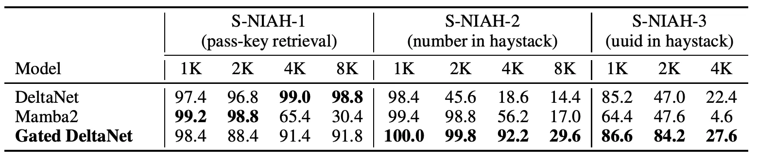
S-NIAH is RULER’s needle-in-haystack suite (Hsieh et al., 2024) RULER: What's the Real Context Size of Your Long-Context Language Models? Hsieh, Sun, Kriman, Acharya, Rekesh, Jia, Zhang, Ginsburg · 2024 arXiv:2404.06654 , with three subtasks: passkey retrieval (S-NIAH-1), number in haystack (S-NIAH-2), and uuid in haystack (S-NIAH-3).

DeltaNet is the right tool for the synthetic passkey (S-NIAH-1) — targeted updates are exactly what precise needle-recall needs, and it stays near-perfect through 8K. But it has no way to clear $S$, so the real-world S-NIAH-2 and -3 trigger the §3 cross-talk story: stored values superimpose as the haystack grows, and accuracy collapses (98.4 → 14.4 from 1K → 8K on S-NIAH-2).

Mamba2 has the opposite problem. Its uniform gate can clear, but it can’t write precisely — so even on the synthetic passkey the needle gets co-decayed with the haystack as context grows (99.2 → 30.4 from 1K → 8K).

Gated DeltaNet pays a small price on synthetic recall (the gate discards information; 8K passkey sits around 90 instead of 99) and wins every cell on S-NIAH-2/3 — precise writes plus the ability to clear.

Both gates depend only on $x_t$ and not on $S_{t-1}$ or the current residual $v_t - S_{t-1} k_t$. They see the input, but not the actual mistake the state is making at $k_t$. A state-aware step size that conditions on the residual would be the natural next step.

Figure 1. Updated:

Model	$A_t$	$b_t$	$\phi$
Softmax	— (no finite $S$)	—	$\exp$ (infinite-dim)
Linear attention	$I$	$v_t$	$\mathrm{elu} + 1$
Mamba2	$\alpha_t\, I$	$v_t$	identity
DeltaNet	$I - \beta_t\, k_t k_t^\top$	$\beta_t\, v_t$	identity
Gated DeltaNet	$\alpha_t\,(I - \beta_t\, k_t k_t^\top)$	$\beta_t\, v_t$	identity

Mamba2 contributes the scalar decay $\alpha_t$; Gated DeltaNet stacks it on the DeltaNet gradient step.

Outlook

So far, every architecture has fit the same recurrence where only $(A_t, b_t)$ varies. We’ve seen two knobs: how we write ($\beta_t$ — the delta rule) and how we forget (decay via $\alpha_t$ — Mamba2 / Gated DeltaNet).

Look back at the move that gave us DeltaNet: one gradient step on $\|v_t - S k_t\|^2$. So $S$ can be viewed as not just a state being updated by a hand-tuned rule, but as a small model being trained as we read. DeltaNet is the special case in which that model has a single linear layer.

Part 2 commits to that view: stop calling $S$ a state, treat it as a tiny model updated online to remember the context. That framing is what opens up TTT, Titans, and the four axes introduced by MIRAS.

References

1. Katharopoulos, Vyas, Pappas, Fleuret (2020). Transformers are RNNs: Fast Autoregressive Transformers with Linear Attention. ICML 2020. arXiv:2006.16236
2. Yang, Wang, Zhang, Shen, Kim (2024). Parallelizing Linear Transformers with the Delta Rule over Sequence Length. NeurIPS 2024. arXiv:2406.06484
3. Dao, Gu (2024). Transformers are SSMs: Generalized Models and Efficient Algorithms Through Structured State Space Duality. ICML 2024. arXiv:2405.21060
4. Yang, Kautz, Hatamizadeh (2024). Gated Delta Networks: Improving Mamba2 with Delta Rule. arXiv:2412.06464
5. Hsieh, Sun, Kriman, Acharya, Rekesh, Jia, Zhang, Ginsburg (2024). RULER: What's the Real Context Size of Your Long-Context Language Models?. arXiv:2404.06654